can we predict cognitive abilities from brain imaging data using conventional (unpenalized) regression ?

This post summarizes the talk that I gave to the study technicians of the Rhineland Study explaining the challenges in predicting cognitive abilities from high-dimensional brain imaging data using conventional (unpenalized) regression, but the ideas here explained apply generally to the modeling of relationships between any input and output data in high dimensions. Conventional regression techniques are not useful in high-dimensional settings. I show how machine learning provides an explanation for this issue and proposes a solution.

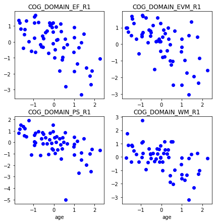
Cognitive abilities can be measured across multiple domains such as working memory, processing speed, episodic verbal memory and executive function. One may wonder how they are determined by factors such as age and sex. One may also wonder how much left is determined by brain structure. To answer these questions, we can use regression analysis to assess the association between cognition and these factors or, put another way, to predict cognition using these factors as input.

To get an idea of the data, we plot different cognitive abilities with respect to age for a subset of participants in the Rhineland Study (variables have been standardized to zero-norm, unit standard deviation).

Let’s define a function that predicts cognition based on age.

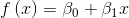
(we are assuming a linear relationship between age and cognition)

In regression analysis, we need a set of examples with pairs of values for age () and cognition (). We estimate the beta coefficients that make up the function as follows:

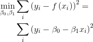
That is, we seek the function f() that predicts with minimum error (ie, squared difference) the cognitive abilities y in our sample. We plot the predictions for our sample in red below. Errors are represented as black lines joining predictions with true values. (we actually compute 4 different functions, one for each cognitive domain)

We see that predictions look like a straight line. This is because we have used a linear function. Based on the slope, we may extract conclusions about the strength of this association. We won’t go into more detail on that here. Let us only note that in general, the greater the magnitude of the beta coefficient (ie, the slope of the line), the more important is the associated factor in the prediction.

To further improve prediction, we may include other factors such as sex.

Adding sex brings the predictions a bit closer to the true values.

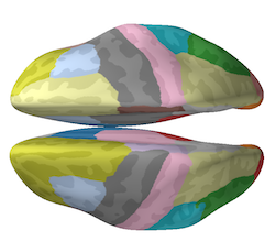
If available, we may further include information about brain structure. Luckily, we have information about thickness across 50+ cortical brain structures in our sample. The cortical brain structures are depicted in different colors in the parcellation below:

Below we show the evolution of the prediction by gradually adding all the available variables, starting by age and sex and following with the cortical thickness measures.

As we include more variables the fit gets better until eventually we obtain perfect prediction in our sample.

At this point we have created 4 functions f() (one for each cognitive domain) that receive age, sex and cortical thickness as input and predict cognitive performance as output. Does this mean that we now exactly predict the cognitive abilities of any person given their age, sex and cortical measures ? Of course not. As a counter-example, consider the how unlikely it is that one participant from our sample would perform exactly the same if they were to repeat the cognitive testing. However, our function would always predict the same value, as long as age, sex and cortical thickness remain constant.

Let us make clear the distinction between learning and prediction.

• Learning involves the creation of the functions relating biological inputs to cognition using an example set of training data
• Predicting means guessing the cognitive performance from the biological inputs, using the functions learned in the previous step

Note that prediction can be done in the same or another dataset as the one used for learning the functions. To see how well the learned functions capture any meaningful relationship, let us predict onto a different set of participants.

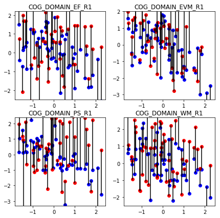
The errors are so large that do not even fit in the plot. What has happened ? With so many inputs, the function is flexible enough to behave in any way we want. As result, it only learns relationships between inputs and output specific to the training data but that do not hold to other participants. In machine learning terms, this is known as overfitting.

To make sure that high-dimensional functions (>10-12 dimensions) capture any meaningful relationship beyond the training dataset, we need to test for generalization. When using only a few variables the function is already constrained enough to be protected against over-fitting (although testing for generalization wouldn’t harm in any case).

To understand this issue consider the following: The true relationship between input and output (if any) hold in any representative sub-set of the data. Therefore, the learning procedure that reveals such true relationship should yield stable models regardless of the training dataset. Highly flexible models contradict this premise by yielding results that depend too much on the particular training set. Note also that, too stable models (eg, a constant function) would also fail for the opposite reason, ie, not explaining anything useful about the data. Therefore, we seek a trade-off between adaptability to the data and stability of the model across training sets. This is known as the bias-variance tradeoff, a central issue in machine learning.

The bias-variance trade-off suggests that we should sacrifice data fitting for the sake of a more stable model across training sets. Although it may not be obvious how allowing for training errors improves generalization, I would argue it is otherwise unreasonable to pursue a perfect fitting for the following reasons:

• missing inputs: we may be missing relevant biological factors that determine cognitive performance
• wrong model assumptions: the relationships between the inputs and outputs in our model (linear in our example) may not be correct
• random errors: the same person may perform differently in the same test for reasons that cannot be determined

Now that I hope I have convinced you, you may ask 1) how we control the degree of flexibility of our function and 2) how to select the appropriate degree ? The first question relates to the topic of regularization. Best-feature-subset selection methods such as the lasso address this issue by restricting the model to only use a sub-set of the inputs.

The second question on how to decide on the appropriate degree of flexibility relates to the topic of model selection. We want to select the model that will perform the best on new data and, for that, we need first to estimate the generalization error. One of the most popular method to estimate the generalization error, and thereby inform model-selection, is cross-validation, which consists in performing learning and prediction in different partitions of the dataset.

In the following, I describe how we go about selecting the model for our problem:

• Partition the dataset in 3 parts for training, validation and test.
• Using the training set, we learn different versions of the model, by varying the degree of complexity (with the lasso).
• Using the validation set, we measure prediction accuracy, ie, how well the model learned on the training data predicts cognition on the validation set
• We select the complexity level with best prediction accuracy on the validation set and re-learn the model using both training and validation sets

Now, we can use the learned model to predict the cognitive performance on the data from the test set, which has not been used at all, and which represents new data that may come in the future. The image below shows the prediction on a test set, by our model selected by the cross-validation procedure above.

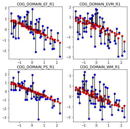
As we can see, age remains the best predictor for cognition, but regularized regression + model selection allowed us to incorporate high-dimensional brain imaging data to refine a bit more the predictions.

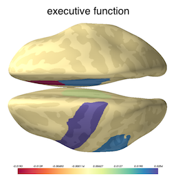
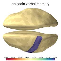
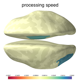
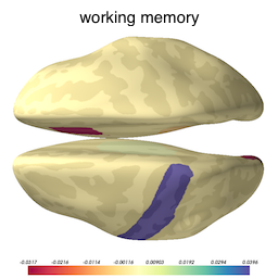
Now that we know our model is not overfitted to the training data, we can inspect the selected variables to ascertain what brain structures got picked up as useful for predicting cognition. The image below shows the brain structures selected by lasso, where blue / red denote respectively that the thickening / thinning of the corresponding structure is associated with higher cognitive performance in each respective domain.