bullseye parcellation of the cerebral white matter with FreeSurfer

In this post I will explain the nits and grits on how to create a bullseye parcellation of the cerebral white matter using (part of) the FreeSurfer outputs and commands. The software package recreating the parcellations according to this post is freely-available in this github repository. So, let’s get started!

The bullseye parcellation that we are aim at creating divides the white matter into a set of concentric regions (ie, layers) spanning from ventricles to cortex that are in turn divided into spatially contiguous regions (ie, lobes). It can be used to obtain region-specific quantification of white matter parameters (eg, a similar approach has been used to quantify regional white matter hyperintensity load in this and this papers).

The image below shows an example bullseye parcellation

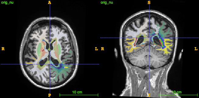
The bullseye parcellation is the intersection of a concentric parcellation dividing the brain into equidistant concentric shells from ventricles to cortex, and a lobar parcellation dividing the brain into its main lobes.

• concentric parcellation

• lobar parcellation

We divide the process into 3 phases:

• lobar parcellation
• concentric parcellation
• bullseye parcellation

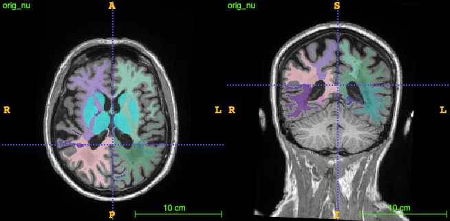
lobar parcellation

We take advantage of FreeSurfer outputs and commands to create the lobar parcellation. We do not need all but only a portion of FreeSurfer outputs. More specifically, from the FS subject directory:

• label/{l,r}h.aparc.annot
• surf/{l,r}h.white
• surf/{l,r}h.pial
• mri/ribbon.mgz
• mri/aseg.mgz

In the first step, we aggregate the cortical parcellation in aparc into a set of lobes with the command:

mri_annotation2label --subject subject --hemi rh --lobesStrict lobes

This command adds the output label/rh.lobes.annot into the FS structure (repeat the command for the left hemisphere lh).

The next step, we need to map the lobes to a volume. This we do with mri_aparc2aseg FS command:

mri_aparc2aseg --s subject --annot lobes --labelwm --wmparc-dmax 1000 --rip-unknown --hypo-as-wm --o lobes+aseg.nii.gz

This creates the volume lobes+aseg.nii.gz containing the projection of the lobar labels into the white matter. A few notes on this command:

• the --labelwm option projects the cortical annotations (in our case the lobes) along the white matter
• the --wmparc-dmax specifies the distance (in mm) that the lobar labels are projected down the white matter. We use a safely large number (ie, 1000) to make sure that we reach the ventricles
• we also remove unknown labels (--rip-unknown) and treat hypointensities as white matter (--hypo-as-wm)

We note here that FS’s definition of lobes is not exactly the same as the one used in the papers above on regional WMH quantification. To improve compatibility, we do some cleaning and re-arranging of labels. In particular, we merge the insular with the frontal lobe and remove a resulting lobe spanning from anterior to posterior in the superior part of the brain (sorry that I do not know the name).

This can be accomplished with the filter_labels.py script from my nimg-scripts repository, as follows (one may as well download the full bullseye package which already does this work for you):

python filter_labels.py --in_dir path/to/lobar/folder/ --in_suffix +aseg.nii.gz --out_dir path/to/output/folder --out_suffix +lobes.nii.gz --include 3001 3007 --include 4001 4007 --include 3004 --include 4004 --include 3005 --include 4005 --include 3006 --include 4006 --map 3001 11 --map 4001 21 --map 3004 12 --map 4004 22 --map 3005 13 --map 4005 23 --map 3006 14 --map 4006 24

Very briefly, we merge the insular (3007, 4007) with frontal (3001, 4001) lobes. We exclude the lobe in the superior part of the brain (3003, 4003). Lastly, we assign informative 2-digit labels to the lobes (--map arguments), with 1st digit denoting the hemisphere and 2nd digit the acutal lobe.

The lobar parcellations are almost (but not yet) ready. Note that we have excluded the lobe 3003, 4003, so we have a hole in its place. Also, there may be regions denoted as unsegmented white matter by FS, which may correspond to, e.g., hypointensities. To fill these regions, we need to do a similar procedure as mri_aparc2aseg with the --labelwm option, consisting on projecting cortical labels into the white matter in the direction from cortex to ventricles. The only difference is that we do not need to go all the way up to the cortex but rather we just need to fill the holes left in the WM by the unsegmented/excluded regions. To that end, we need to know, for each point in the WM, what next point to visit to go in the direction from cortex to ventricles. We accomplish this using a so-called normalized distance map, which will be also useful for computing the depth parcellations at a later stage.

normalized distance map

We call normalized distance map, a map defined in the image, with the characteristics that its value is 0 on the ventricles, 1 on the cortex and smoothly interpolates in-between. Here I show one example:

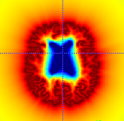
(we can easily discard values outside our region of interest with a WM mask)

It can be easily created in Python with the following 5 lines of code:

import numpy as np
from scipy.ndimage.morphology import distance_transform_edt

dist_orig = distance_transform_edt(np.logical_not(ventricle_mask))
dist_dest = distance_transform_edt(np.logical_not(cortex_mask))
ndist = dist_orig / (dist_orig + dist_dest)

The idea is to create two distance maps, with each voxel denoting the distance to a mask of interest, in our case the ventricle_mask and cortex_mask, respectively. The normalized distance map is then the distance from the ventricles divided by the sum of distances from the ventricles and cortex. Note that this is 0 in the ventricles, 1 in the cortex and smoothly interpolates in-between. You can see how this will make straightforward the computation of the depth parcellations later.

Back to the lobar parcellations, we fill the WM holes, as follows:

• set ID to 0
• sort all voxels wrt their normalized distance in a priority queue
• while there are unlabeled voxels:
  • pop next voxel
  • if it is not labeled:
    • ID = ID + 1
    • label the voxel with ID and all the voxels along the gradient trace to the cortex (the gradient is straightforward with the distance map)
    • when reaching the cortex create a look-up table ID -> cortex label
• iterate over all voxels and replace ID with corresponding cortex label in the lookup table

Voila! we know how to project the labels to fill the WM holes.

Finally, we include the subcortical structures in the basal ganglia + thalami as another additional lobe. This simply amounts to assigning their corresponding FS IDs in aseg (i.e., 10, 49, 11, 12, 50, 51, 26, 58, 13, 52) to a single ID (we use 5), and then merging the resulting mask with the lobar parcellation.

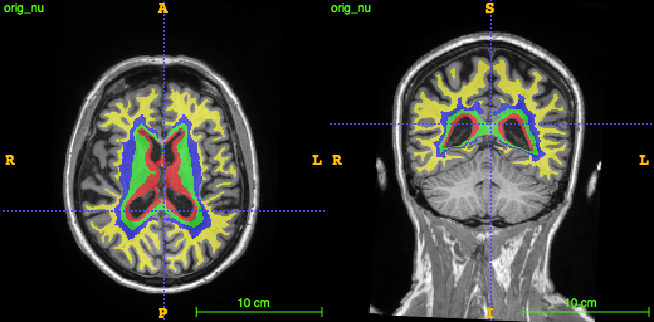
depth parcels

We can straightforwardly get a depth parcellation with the normalized distance map as follows:

import numpy as np

out = np.zeros(ndist.shape, dtype=np.int8)

limits = np.linspace(0., 1., n_shells+1)
for i in np.arange(n_shells)+1:
    # compute shell and assing increasing label-id
    mask = np.logical_and(ndist >= limits[i-1], ndist < limits[i])
    out[mask] = i
out[np.isclose(ndist, 0.)] = 0  # need to assign zero to ventricles because of >= above

where ndist is the normalized distance map and n_shells is the number of desired parcels (4 in our case).

bullseye parcellation

Finally, we create the bullseye parcellation by intersecting the lobar and depth parcels as follows:

import numpy as np

out = np.zeros(lobes.shape, dtype=np.int32)

u1_set = np.unique(lobes.ravel())
u2_set = np.unique(depth.ravel())

for u1 in u1_set:
    if u1 == 0: continue
    mask1 = lobes == u1
    for u2 in u2_set:
        if u2 == 0: continue
        mask2 = depth == u2
        mask3 = np.logical_and(mask1, mask2)
        if not np.any(mask3): continue
        out[mask3] = int(str(u1) + str(u2))  # new label id by concatenating [u1, u2]

where lobes and depth contain the lobar and depth parcels, respectively. For easy interpretation, we generate the labels IDs of each bullseye parcel as concatenation of the lobar and depth IDs.

I hope that this tutorial was helpful. You can download and use the package to create the bullseye parcellations in this github repository.